How to Create and Use Sparkline Charts in Presentations

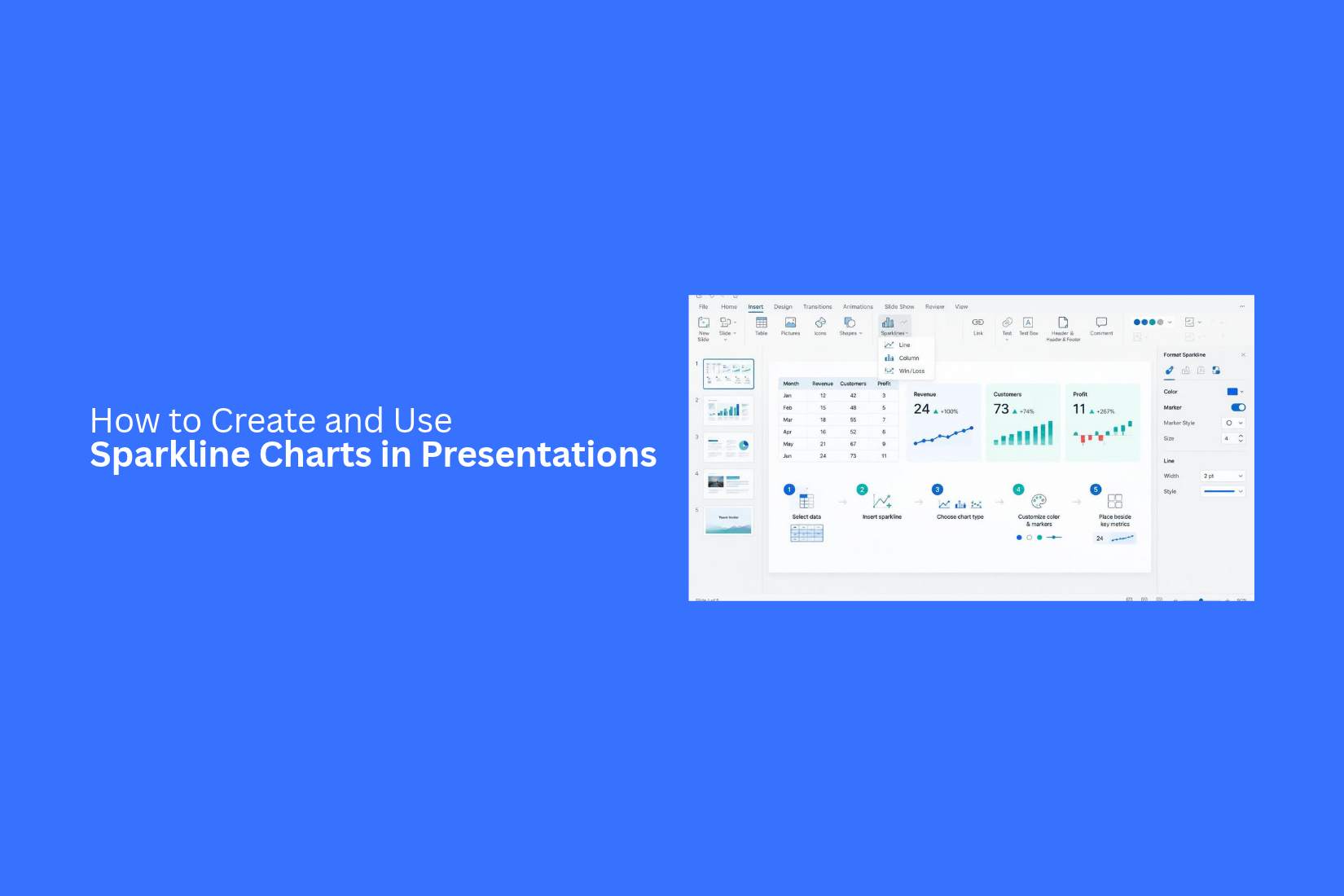
Data plays a key role in business presentations. However, large charts can take up too much slide space. They can also make it harder for viewers to spot key trends. This can leave important details hidden among rows of numbers and complex visuals.

A crowded slide can distract your audience. It may also take more time to explain simple changes in sales, revenue, or business performance. As a result, your main message may get less attention.

Sparkline charts offer a simple way to present data trends in a small space. In this guide, you'll learn how to create and customize sparklines in Excel and Google Sheets. You'll also learn how to add them to PowerPoint and Google Slides, use them in business reports, and design clear data-focused slides.

What Is a Sparkline Chart?

A sparkline chart is a small chart that shows data trends in a simple way. It usually appears inside a text box, table cell, or next to a key number. Unlike regular charts, sparklines do not need axes, labels, or legends. They focus on the main data pattern.

You can use sparkline charts to show changes over time. For example, a sales report can use a small line chart to show monthly sales growth. A financial report can use one to show changes in stock prices. These small charts help readers understand data without taking up much slide space.

Sparkline charts are useful for business reports, financial presentations, dashboards, and performance reviews. They let you compare several data sets on one slide. This makes it easier to spot trends and review key numbers at a glance.

Different Types of Sparkline Charts

Sparkline charts come in three main types: line, column, and win/loss. Each type shows data in a different way. The right choice depends on the information you want to share. Some work best for showing trends over time. Others help compare values or track positive and negative results.

Line Sparklines

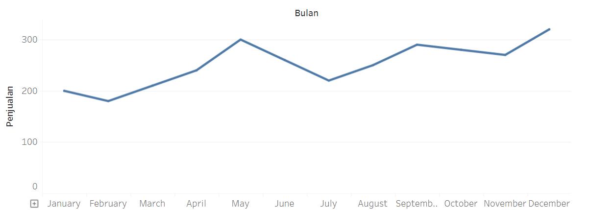
Line sparklines use a simple line to show changes in data. They connect data points in order. This makes it easy to see whether values are rising, falling, or staying close to the same level.

For example, a line sparkline can show monthly sales over one year. A rising line shows sales growth. A falling line points to a drop in sales. Small changes appear as peaks and dips along the line.

 Line sparklines work well for:

 • Tracking sales or revenue over time.

 • Showing website traffic changes.

• Monitoring monthly expenses.

• Comparing performance trends.

• Displaying changes in user activity.

Column Sparklines

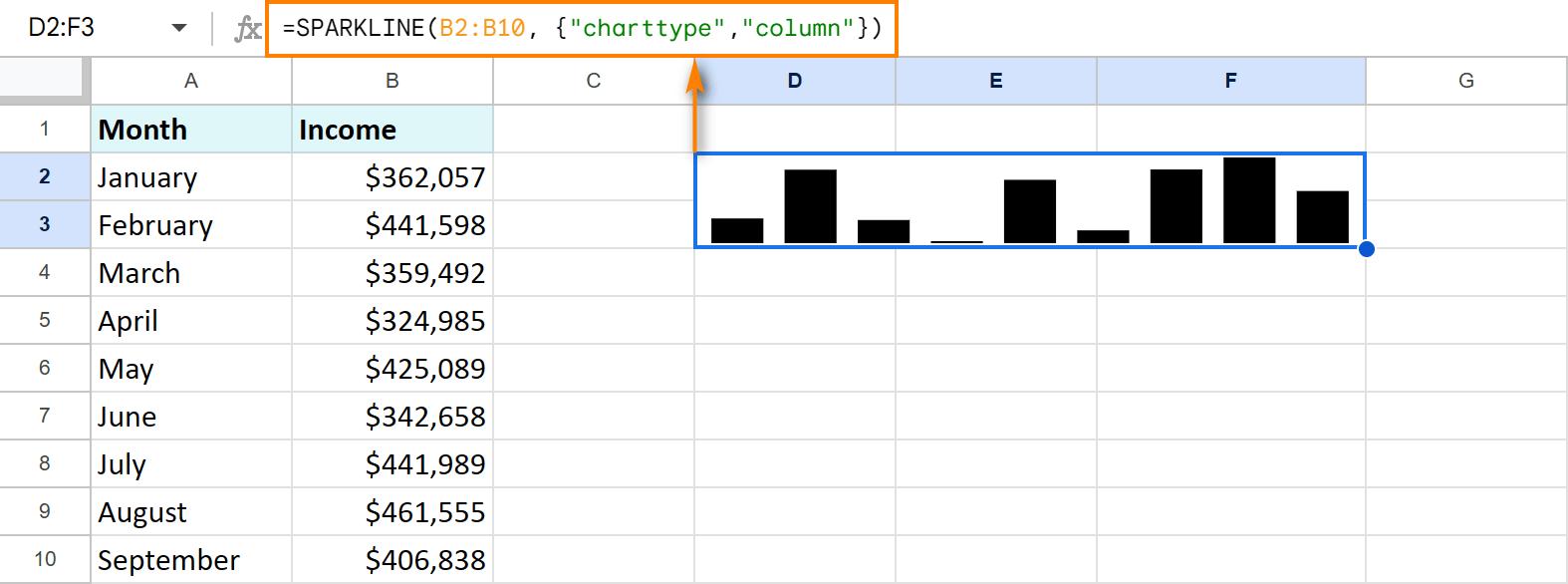
Column sparklines use vertical bars to show data values. Each bar represents one value in a data series. Taller bars show higher values. Shorter bars show lower values.

This type makes it easier to compare values across different periods. For example, a column sparkline can show monthly sales for a year. The bars help viewers spot the months with the highest and lowest sales.

Column sparklines work well for:

• Comparing monthly sales figures.

• Tracking quarterly revenue.

• Showing weekly website visits.

• Comparing production levels.

• Displaying changes in monthly expenses.

You can also use different colors to mark specific bars. A different color for the highest or lowest value can help draw attention to key results.

Win/Loss Sparklines

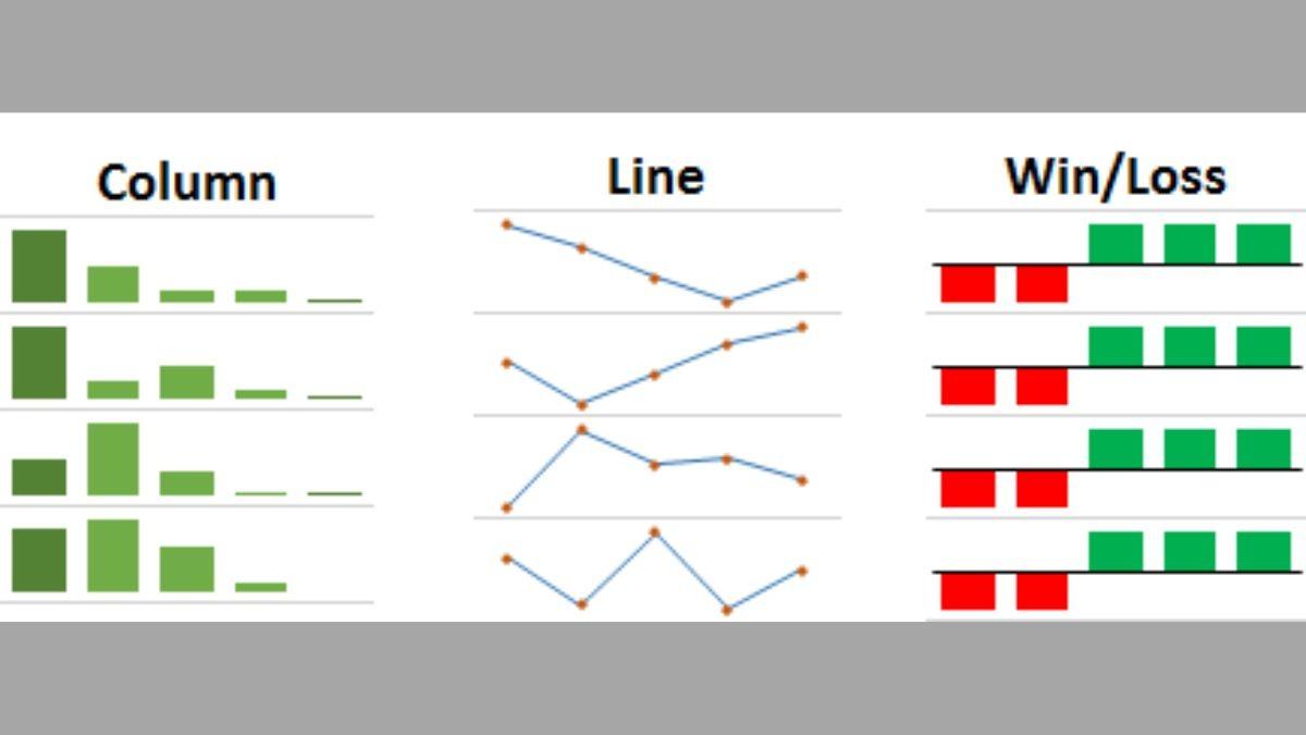
Win/loss sparklines show positive and negative results. They use bars above or below a center line. Positive results appear above the line. Negative results appear below it. Equal or zero values may appear as flat marks. Unlike line and column sparklines, this type does not focus on the size of each value. It shows the direction of the result. This makes it useful for tracking wins and losses over a set period.

For example, a win/loss sparkline can show a sports team's results across several games. It can also track monthly profit and loss or compare sales targets with actual results.

Win/loss sparklines work well for:

• Tracking wins and losses in sports.

• Showing monthly profit or loss.

• Monitoring sales target results.

• Comparing positive and negative performance.

• Tracking project milestones.

How to Choose the Right Sparkline Type

Each sparkline type serves a different purpose. Your choice should match the data and the message of your presentation.

Use these simple guidelines:

• Choose line sparklines to show trends over time. They work well for sales growth, website traffic, and other changing values.

• Choose column sparklines to compare values across periods. They are useful for monthly sales, quarterly revenue, and production data.

• Choose win/loss sparklines to show positive and negative results. They work well for profit and loss reports, sports results, and target tracking.

The amount of detail also matters. A line sparkline shows the overall direction of data. A column sparkline makes value differences easier to see. A win/loss sparkline gives a quick view of results. Keep your audience in mind. Pick the chart type that helps them understand the data at a glance.

How to Create Sparkline Charts in Excel

Excel makes it easy to create sparkline charts. You can add small charts inside individual cells to show changes in your data. These charts work well for sales reports, financial summaries, and presentation tables. Excel offers three main sparkline types: Line, Column, and Win/Loss. Let's go through each type and see how to create it.

Prepare Your Data for Sparklines

Start by arranging your data in a clear table. Each row should contain one set of values that you want to display in a sparkline.

For example, a sales report may show monthly sales for several products. Each product gets its own row, with sales figures from January to December.

Follow these steps:

1. Open your Excel worksheet.
2. Enter your data in rows or columns.
3. Add a label for each data set.
4. Keep the values in a consistent order.
5. Select an empty cell where you want the sparkline to appear.

A clear data layout makes it easier to create and read your charts. Leave enough space for the sparkline cells beside your data.

Create Line Sparklines

Line sparklines show trends over time. They connect data points with a line. This makes them useful for tracking monthly sales, website traffic, or yearly revenue.

Here is how to create one:

1. Select the cell where you want the sparkline.
2. Open the Insert tab in Excel.
3. Find the Sparklines group.
4. Click Line.
5. In the Create Sparklines window, select your data range.
6. Check the Location Range field.
7. Click OK.

Excel will add a small line chart inside the selected cell. You can also use the Sparkline tab to change its color, show data markers, and highlight high or low points.

Create Column Sparklines

Column sparklines use vertical bars to show changes in data. Each bar represents one value. Taller bars show higher values, while shorter bars show lower values.

This type works well for comparing monthly sales, product performance, or quarterly revenue.

Follow these steps:

1. Select an empty cell for your sparkline.
2. Go to the Insert tab.
3. Click Column in the Sparklines group.
4. Select the data range you want to display.
5. Check the location range.
6. Click OK.

Excel will place a small column chart inside the selected cell. You can change the bar color and highlight the highest or lowest values from the Sparkline tab.

Create Win/Loss Sparklines

Win/Loss sparklines show positive and negative results. They use bars of equal height to mark wins and losses. Positive values appear above the center line, while negative values appear below it.

This chart type works well for profit and loss reports, sales targets, and sports results.

Here is how to create one:

1. Select the cell where you want the chart.
2. Open the Insert tab.
3. Click Win/Loss in the Sparklines group.
4. Select your data range.
5. Confirm the location range.
6. Click OK.

Excel will create a small chart that shows positive and negative results. You can use the Sparkline tab to change the colors and highlight key points.

Create Multiple Sparklines at Once

Creating sparklines one by one can take extra time. Excel lets you create several sparklines in one step. This is useful for reports with many products, regions, or sales teams.

For example, a table may contain monthly sales data for five products. You can create five line sparklines at once to compare their sales trends.

Follow these steps:

1. Arrange each data set in a separate row.
2. Select the full range of data.
3. Open the Insert tab.
4. Choose Line, Column, or Win/Loss from the Sparklines group.
5. In the Create Sparklines window, select the full range of data.
6. Select the matching number of empty cells in the Location Range field.
7. Click OK.

Excel will create one sparkline for each row of data. Each chart will appear in its matching cell. This method saves time and keeps your worksheet organized. It also makes it easier to compare several data sets before adding them to a presentation.

How to Customize Sparkline Charts in Excel

Excel lets you change the look of sparkline charts. You can adjust their colors, highlight key data points, and change axis settings. These options help you make each chart easier to read. They also help you match the chart with your presentation theme.

Change Sparkline Colors and Styles

Color changes can make a sparkline easier to read. Excel provides several color options for lines and columns. You can also adjust the line width to make a line sparkline more visible.

Follow these steps to change the color and style:

1. Select the cell that contains your sparkline.
2. Open the Sparkline tab in the ribbon.
3. Click Sparkline Color to change the line or column color.
4. Choose a color from the available options.
5. Click Marker Color to change the color of data markers.
6. Use the Weight option to adjust the line thickness.

Excel also offers built-in styles. Select a style from the Style group to apply a different look. Choose colors that match your presentation theme. Keep enough contrast between the sparkline and its background.

Highlight High, Low, First, and Last Points

A sparkline shows data trends in a small space. Some points may need extra attention. Excel lets you highlight the highest, lowest, first, and last values.

These markers help viewers spot key changes without reading every value.

To highlight these points:

1. Select the sparkline cell.
2. Open the Sparkline tab.
3. Find the Show group.
4. Check High Point to mark the highest value.
5. Check Low Point to mark the lowest value.
6. Check First Point to mark the starting value.
7. Check Last Point to mark the ending value.

You can also enable Negative Points to mark values below zero. Use the Marker Color menu to assign different colors to these points. This makes key values stand out in your presentation.

Adjust Horizontal and Vertical Axis Settings

Axis settings control how Excel displays values in a sparkline. These settings can affect how viewers read changes in your data.

For example, two sparklines may show the same values but look different because they use different vertical scales. A shared scale makes it easier to compare trends across several rows.

Follow these steps to adjust the axis:

1. Select the sparkline or group of sparklines.
2. Open the Sparkline tab.
3. Click Axis in the Group section.
4. Choose Vertical Axis Minimum Value to set the lowest value.
5. Choose Vertical Axis Maximum Value to set the highest value.
6. Select Same for All Sparklines to use one scale across the selected charts.

You can also adjust the horizontal axis. Excel lets you show dates or set how empty cells affect the chart. These options help keep the data in the correct order.

Display Negative Values and Empty Cells

Negative values and empty cells can affect how a sparkline looks. Excel provides settings to control how these values appear.

For example, a sales report may include both positive and negative values. Showing negative points helps viewers spot periods with losses.

To display negative values:

1. Select the sparkline cell.
2. Open the Sparkline tab.
3. Check Negative Points in the Show group.
4. Open Marker Color and select Negative Points.
5. Choose a color that makes negative values easy to spot.

Excel also lets you control how empty cells appear in a sparkline.

1. Select the sparkline.
2. Open the Sparkline tab.
3. Click Edit Data.
4. Select Hidden & Empty Cells.
5. Choose how Excel should display empty cells:

• Gaps: Leaves a blank space in the chart.

• Zero: Treats empty cells as zero values.

• Connect data points with line: Draws a line across empty cells in a line sparkline.

These settings help keep your charts clear. Pick the option that best matches your data. For presentation slides, use clear markers and colors so viewers can read the trend at a glance.

How to Add Sparkline Charts to PowerPoint Presentations

Excel makes it easy to create sparkline charts, but PowerPoint does not have a dedicated sparkline feature. You can still add these small charts to your slides by using a few different methods. Each method offers a different level of control over editing and updates.

Copy and Paste Sparklines from Excel

Copying sparklines from Excel is one of the easiest ways to add them to PowerPoint. You can create the chart in Excel, copy it, and paste it directly onto a slide.

Follow these steps:

1. Open your Excel file and select the cell containing the sparkline.
2. Press Ctrl + C to copy it.
3. Open your PowerPoint presentation and select the slide.
4. Press Ctrl + V to paste the sparkline.
5. Resize and position the chart to fit your slide layout.

PowerPoint may offer different paste options. Choose Use Destination Theme to match the presentation style or Keep Source Formatting to retain the original Excel appearance.

Insert Sparklines as Pictures

Pasting a sparkline as an image keeps its appearance fixed. This option works well for slides that need a clean layout without further chart editing.

To insert a sparkline as a picture:

1. Select the sparkline in Excel.
2. Copy it using Ctrl + C.
3. Open PowerPoint and go to the Home tab.
4. Click the arrow under Paste.
5. Select Picture from the paste options.

You can also use Excel's Copy as Picture feature to copy the sparkline as an image. Once inserted, the sparkline behaves like any other picture. You can crop it, resize it, rotate it, or apply picture formatting. However, changes to the original Excel data will not update the image.

Use Linked Pictures to Keep Sparklines Updated

A linked picture connects the sparkline in PowerPoint to its original Excel file. This lets the presentation reflect changes made to the source chart after the link is updated.

Here is how to create one:

1. Select the sparkline in Excel.
2. Copy it using Ctrl + C.
3. Open PowerPoint and select the target slide.
4. Go to Home and open the Paste dropdown.
5. Select Paste Special.
6. Choose Paste Link and select a picture format, if available.
7. Click OK.

Now, PowerPoint keeps a link to the Excel source. Updates to the source file can appear in the presentation after the link is refreshed. Keep the original Excel file in the same location. Moving or renaming it may break the link. Linked pictures also depend on access to the source file, so they may not update properly after sharing the presentation.

Recreate Sparklines Using PowerPoint Charts

Another option is to build a small chart directly in PowerPoint. This gives you more control over its appearance and data without relying on an external Excel file.

Follow these steps:

1. Open your PowerPoint slide.
2. Go to Insert > Chart.
3. Select a Line or Column chart.
4. Enter your data in the Excel sheet that opens.
5. Close the data sheet after entering the values.
6. Remove the chart title, legend, gridlines, and other unnecessary elements.
7. Adjust the chart size and formatting to create a sparkline-style visual.

A regular PowerPoint chart may include more elements than a true sparkline. Removing these elements helps create a compact chart that shows a simple data trend. You can also change the line color, marker style, and axis settings to match your presentation design.

Resize and Position Sparklines on Slides

The size and placement of a sparkline affect how easily viewers can read it. A small chart should support the nearby content without taking too much space.

Use these tips to place sparklines neatly:

• Keep a consistent size: Use similar dimensions for sparklines that appear in the same slide or across multiple slides.

• Maintain clear spacing: Leave enough room between the chart and nearby text, icons, or other visuals.

• Align with related content: Place each sparkline beside its matching metric, heading, or data label.

• Preserve proportions: Drag a corner handle to resize the chart without stretching it.

• Use readable colors: Choose line and column colors that stand out against the slide background.

• Avoid unnecessary details: Remove extra borders, labels, and visual elements that take attention away from the trend.

For a dashboard-style slide, place each sparkline beside the number or category it represents. This helps viewers connect the data trend with the key figure without reading a large chart.

How to Create Sparkline Charts in Google Sheets

Google Sheets lets you create small charts inside individual cells. These charts are called sparklines. They show data trends in a compact format. You can use them to track sales, compare monthly results, or show changes over time. The SPARKLINE function makes this process simple. You can also change the chart type, color, and other settings to match your data. Let's go through the steps.

Prepare Data for Sparkline Formulas

Start by arranging your data in Google Sheets. Keep the values you want to show in a row or column. For example, you can use monthly sales data for one product.

Here is a simple example:

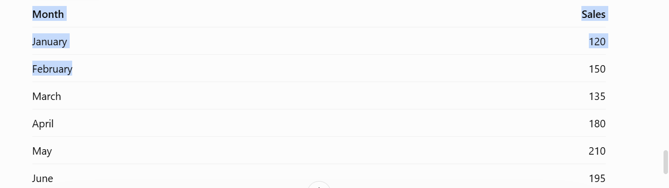
Place the months in one column and the sales values in another. This layout makes it easy to select the right data range.

Next, choose an empty cell for your sparkline. The chart will appear inside that cell. Make sure the cell has enough width and height to show the chart clearly.

Create Sparklines Using the SPARKLINE Function

Google Sheets uses the SPARKLINE function to create small charts inside cells. You only need to select the data range.

Follow these steps:

1. Open your Google Sheets file.
2. Find the data you want to display as a sparkline.
3. Select an empty cell next to your data.
4. Enter the following formula:

=SPARKLINE(B2:B7)

5. Press Enter.

Google Sheets will create a small line chart inside the selected cell. The chart shows how the values change across the selected range.

You can copy the formula to other cells. This helps you create sparklines for multiple rows of data. Just make sure each formula points to the correct range.

Customize Sparkline Types and Colors

A basic sparkline uses a line chart. Google Sheets also lets you change its type and color. You can use these options to match the chart with your data.

For example, use a column chart to compare values. A win-loss chart works well for showing positive and negative results.

To create a column sparkline, use this formula:

=SPARKLINE(B2:B7, {"charttype","column"})

To change the line color, use this formula:

=SPARKLINE(B2:B7, {"color","blue"})

You can also combine both settings in one formula:

=SPARKLINE(B2:B7, {"charttype","column";"color","green"})

Here are some common sparkline options:

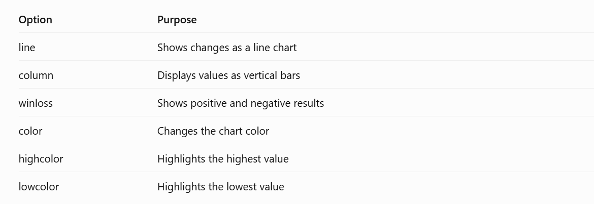
These settings help you make each sparkline easier to read. Use colors that work well with your presentation theme.

Add Google Sheets Sparklines to Google Slides

Once your sparklines are ready, you can add them to Google Slides. This helps you use live data trends in your presentation.

Follow these steps:

1. Open your Google Sheets file.
2. Select the cells that contain your sparklines.
3. Copy the selected cells.
4. Open your Google Slides presentation.
5. Select the slide where you want to add the charts.
6. Paste the copied content.
7. Choose the linking option if you want to connect the pasted content to the original spreadsheet.

Linked content can be updated from Google Sheets. This helps keep your presentation data in sync with the source file. You can also adjust the size and position of the pasted content. Place the sparklines near the related text or data table. This gives your audience a clear view of the trends without taking up too much slide space.

How to Use Sparkline Charts in Presentations

Sparkline charts help you show data trends in a small space. They work well in business reports, financial updates, and marketing presentations. You can place them beside numbers or inside a table. This makes it easier for your audience to see changes over time.

Here are five ways to use sparklines in your presentations.

Show Monthly Sales and Revenue Trends

Monthly sales and revenue data can be hard to read in a large table. A sparkline makes the trend easier to follow. You can use it to show sales changes across several months.

For example, add a sparkline beside your monthly sales figures. Your audience can quickly see which months had higher or lower sales. This also helps show seasonal changes and sales patterns.

Compare Business Performance Across Regions

A business may operate in several regions. Each region may have different sales figures and growth rates. A sparkline can help compare these changes in one view. Add a separate sparkline for each region. Place them beside the region names or sales figures. This lets your audience compare performance without viewing several large charts. It also helps show which regions are growing or losing sales.

Track Financial Growth and Losses

Financial reports often include data from several months or years. A sparkline can show how financial results change over time. You can use one to track revenue, expenses, profit, or losses. Place the chart beside the related figures. This gives your audience a quick view of financial performance. It also helps them spot periods of growth or decline.

Present Marketing Campaign Results

Marketing teams track several results to measure campaign performance. These may include website visits, clicks, leads, and conversions. A sparkline can show how each metric changes over time.

For example, use one sparkline to show daily website traffic. Add another to track leads from the same campaign. Your audience can compare the trends without reading a long list of numbers. This makes campaign reports easier to follow.

Monitor Key Performance Indicators (KPIs)

KPIs help teams measure progress toward business goals. Common examples include sales growth, customer retention, website traffic, and conversion rates. You can add a sparkline beside each KPI. This shows how the metric changes over a set period. Your audience can spot rising or falling trends at a glance. It also helps them compare current results with past performance.

Sparkline Chart Examples for Business Presentations

Sparkline charts work well in business presentations. They show data trends in a small space. You can add them to reports, dashboards, and summary slides. Each sparkline can show changes over time without taking up much room. Here are four ways to use them in business slides.

Sales Performance Dashboard

A sales dashboard can use sparklines to show changes in sales over time. You can place a small chart beside each sales metric. For example, one sparkline can show monthly revenue. Another can track the number of orders or new customers.

This layout helps viewers check several sales trends at once. They can spot rising or falling numbers with a quick look. It also keeps the dashboard clean and easy to read.

Financial Performance Report

Financial reports often include data for several months or years. Sparklines can show trends in revenue, expenses, profit, and cash flow. You can place each chart beside its related figure.

For example, a revenue sparkline can show monthly income over a year. An expense sparkline can show how costs changed during the same period. These small charts help readers compare financial trends without adding large charts to the slide.

Marketing Analytics Slide

Marketing teams track many metrics across campaigns. These may include website visits, clicks, leads, and conversions. Sparklines can show how each metric changes over time.

You can place a sparkline next to each key number. A website traffic chart may show a rise in visits after a campaign launch. A conversion chart may show whether more visitors became customers. This makes it easier to review campaign results on one slide.

Business KPI Summary

A KPI summary slide gives a quick view of business performance. Sparklines can help show trends for key metrics such as customer growth, sales targets, profit margins, and employee productivity.

Place each sparkline beside its KPI value. You can also add a short label to show the time period. This gives viewers both the current result and its recent trend. They can review several business goals without reading a large table.

Best Practices for Designing Sparkline Charts

A good sparkline chart should be easy to read. It should help your audience spot trends without taking up too much space. A few simple design choices can make your sparklines more useful. Follow these best practices to keep your charts clear and easy to understand.

Keep Sparklines Close to Their Related Data

Place each sparkline next to the data it represents. This helps your audience connect the chart with the right numbers. For example, add a sparkline beside a sales total or monthly revenue figure. Keep the chart and its data in the same row or table cell.

Avoid placing sparklines far from their related values. Your audience may have trouble finding the right data. A clear layout makes the chart easier to read.

Use Consistent Scales for Comparisons

Use the same scale for sparklines that show similar data. This makes it easier to compare trends across products, teams, or time periods.

For example, two sales sparklines should use the same vertical scale. A shared scale helps your audience spot differences in performance. Different scales may make small changes look much larger than they are.

Choose Colors That Improve Readability

Use colors that make each sparkline easy to read. A dark line on a light background often works well. Keep the color choices simple and consistent across your slides.

You can also use color to show different data types. For example, use blue for regular trends and red for a drop in sales. Make sure the colors stand out from the background. Avoid using too many colors in one chart.

Highlight Important Trends

Use markers or a different line color to draw attention to key data points. You can highlight the highest value, lowest value, or last value in a series.

For example, a sales sparkline may show a sharp drop in the final month. A red marker can help your audience spot that change. Keep the highlight clear. Too many markers can make the chart harder to read.

Avoid Adding Too Much Data to One Sparkline

A sparkline works best with a small set of related data. Too many data points can make the line look crowded. Small changes may also become hard to see.

Choose the data that supports your main point. For example, use monthly sales figures for a one-year trend. Avoid mixing unrelated values in the same sparkline. Split the data into separate charts if you need to show more than one trend.

Common Sparkline Chart Problems and How to Fix Them

Sparkline charts are small, but a few issues can affect how they look and work in a presentation. Lines may change after copying. Linked data may stop updating. Some trends may also be hard to read. Here are some common problems and simple ways to fix them.

Sparklines Look Different After Copying to PowerPoint

A sparkline may look different after you copy it from Excel to PowerPoint. The line color, size, or markers may change. This can happen due to differences in formatting between the two apps.

To keep the chart looking the same, use the Paste Special option in PowerPoint. You can paste the sparkline as an image to keep its original look. However, you will not be able to edit the chart data in PowerPoint. You can also paste it as an Excel object. This keeps the chart editable. Check the size and style after pasting. Make small changes to match the rest of your slides.

Linked Sparklines Do Not Update

Linked sparklines may stop updating after you change the source data. This can happen if the file location changes or the link breaks. Start by checking the Excel file. Make sure the source data is still in the same location. Open PowerPoint and check the link settings. Update the links if needed. You can also open the source Excel file and save your changes. Then return to PowerPoint and refresh the linked content. Keep both files in a stable folder to avoid broken links.

Sparkline Lines and Markers Are Difficult to See

Small sparkline charts can be hard to read on a presentation slide. Thin lines may blend into the background. Small markers may also be hard to spot. Use a darker line color with enough contrast against the slide background. Increase the line weight to make the chart easier to see. You can also highlight key data points with markers. Avoid using too many colors. A simple color scheme helps the audience follow the trend. Make sure the chart is large enough to read from a distance.

Data Trends Look Misleading Because of Axis Scaling

Axis scaling can change how a sparkline looks. A small change in data may appear large if the vertical axis has a narrow range. A wide range can make major changes look small. Check the axis settings before adding the chart to your slide. Use the same vertical axis range for sparklines that you want to compare. This makes it easier to spot differences between data sets. You can also set a minimum and maximum axis value. Keep the scale consistent across related charts. This helps your audience read the data correctly.

Final Notes

Sparkline charts help you present data trends in a small space. They work well for sales reports, financial updates, marketing analytics, and business dashboards. You can use line, column, or win/loss sparklines to show different types of results.

Excel and Google Sheets make it easy to create and customize these charts. You can change colors, highlight key data points, and adjust axis settings. You can also add sparklines to PowerPoint and Google Slides to make your slides more useful.

Keep your charts simple and easy to read. Place each sparkline near its related data. Use consistent scales for comparisons. Choose colors with enough contrast. These small design choices help your audience understand key trends without reading large tables or charts.

Frequently Asked Questions (FAQs)

1. What is a sparkline chart?

A sparkline chart is a small chart that shows data trends. It usually appears inside a table cell or next to a key number. It helps viewers understand changes without using a large chart.

2. What are the three main types of sparkline charts?

The three main types are line, column, and win/loss. Line sparklines show trends over time. Column sparklines compare values. Win/loss sparklines show positive and negative results.

3. Can I create sparkline charts in Excel?

Yes. Excel has a built-in Sparkline feature. You can create line, column, and win/loss charts from the Insert tab. You can also change colors, highlight key points, and adjust axis settings.

4. How do I create a sparkline chart in Google Sheets?

You can use the SPARKLINE function in Google Sheets. Select an empty cell and enter a formula such as =SPARKLINE(B2:B7). Press Enter to create the chart.

5. Can I add sparkline charts to PowerPoint?

Yes. You can copy sparklines from Excel and paste them into PowerPoint. You can also insert them as pictures, use linked pictures, or create small charts directly in PowerPoint.

6. Can I use sparkline charts in Google Slides?

Yes. You can copy sparkline cells from Google Sheets and paste them into Google Slides. You can also choose the linking option to connect the content to the original spreadsheet.

7. How do I keep sparkline charts updated in PowerPoint?

Use the Paste Special option and select Paste Link to connect the sparkline to its Excel source. Keep the original file in the same location. You can refresh the link in PowerPoint to show the latest data.

8. What is the best way to make sparkline charts easier to read?

Use clear colors, readable line widths, and consistent scales. Place each sparkline near its related data. Highlight key values with markers. Avoid adding too many data points to one chart.